CS231n 作业一:k-近邻 (kNN) 练习题
k-近邻 (kNN) 练习题
完成并提交这份工作表(包括输出和外部支持代码)。更多信息,详见课程网站。
kNN 分类器包含两个阶段:
- 训练阶段,分类器取出训练数据,并简单的记住他们;
- 测试阶段,kNN 会将测试图像与所有训练图像进行比较,取出 k 个最相似的训练图,并找到出现频率最高的标签;
- k 的取值是通过交叉验证来确定的。
在本练习中,你会实现上述步骤,从而理解图像分类的基本流程和交叉验证的方法,并熟练掌握编写高效的向量化代码的方法。
# 给这个 notebook 运行一些启动代码

import random
import numpy as np
from cs231n.data_utils import load_CIFAR10
import matplotlib.pyplot as plt

# 这是 notebook 的 magic 命令,可以让 matplotlib 的图表
# 显示在 notebook 中,而不是在一个新窗口里边
%matplotlib inline
plt.rcParams['figure.figsize'] = (10.0, 8.0) # set default size of plots
plt.rcParams['image.interpolation'] = 'nearest'
plt.rcParams['image.cmap'] = 'gray'

# 还是一些 magic 命令,让 notebook 重载外部的 python 模块;
# 见:http://stackoverflow.com/questions/1907993/autoreload-of-modules-in-ipython
%load_ext autoreload
%autoreload 2
# 加载原始 CIFAR-10 数据
cifar10_dir = 'cs231n/datasets/cifar-10-batches-py'

# 清理变量,以防多次加载数据(这可能会导致内存问题)
try:
   del X_train, y_train
   del X_test, y_test
   print('Clear previously loaded data.')
except:
   pass

X_train, y_train, X_test, y_test = load_CIFAR10(cifar10_dir)

# 完整性测试,打印训练集和测试集的大小
print('Training data shape: ', X_train.shape)
print('Training labels shape: ', y_train.shape)
print('Test data shape: ', X_test.shape)
print('Test labels shape: ', y_test.shape)
Training data shape:  (50000, 32, 32, 3)
Training labels shape:  (50000,)
Test data shape:  (10000, 32, 32, 3)
Test labels shape:  (10000,)
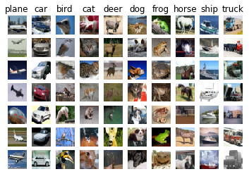
# 可视化数据集中的一些用例
# 每种类型显示几张训练集中的图片
classes = ['plane', 'car', 'bird', 'cat', 'deer', 'dog', 'frog', 'horse', 'ship', 'truck']
num_classes = len(classes)
samples_per_class = 7
for y, cls in enumerate(classes):
    idxs = np.flatnonzero(y_train == y)

    idxs = np.random.choice(idxs, samples_per_class, replace=False)

    for i, idx in enumerate(idxs):
        plt_idx = i * num_classes + y + 1
        plt.subplot(samples_per_class, num_classes, plt_idx)
        plt.imshow(X_train[idx].astype('uint8'))
        plt.axis('off')
        if i == 0:
            plt.title(cls)
plt.show()
# 作为练习,为了避免运行时间太长,这里再对数据进行采样,减小规模
num_training = 5000
mask = list(range(num_training))
X_train = X_train[mask]
y_train = y_train[mask]

num_test = 500
mask = list(range(num_test))
X_test = X_test[mask]
y_test = y_test[mask]

# 把图片数据变成一行 (32, 32, 3) -> 3072
X_train = np.reshape(X_train, (X_train.shape[0], -1))
X_test = np.reshape(X_test, (X_test.shape[0], -1))
from cs231n.classifiers import KNearestNeighbor

# 创建 KNN 分类器实例
# 注意训练 KNN 分类器其实什么也没干,分类器只是简单地记录了一下数据
classifier = KNearestNeighbor()
classifier.train(X_train, y_train)
现在,我们要用 KNN 分类器对测试用例进行分类。回想一下,我们可以将该过程分为两个步骤:
- 首选,我们计算测试用例与所有训练示例的距离;
- 得到这些距离之后,对于每个测试用例,找到 K 个最邻近的示例(每个示例都有一个对应的标签),并从中选出票数最高的标签。
让我们从计算所有训练示例和测试用例之间的距离开始。举个🌰,如果有 Ntr 个训练示例和 Nte 个测试用例,这个阶段应该返回一个 Nte x Ntr 的矩阵,矩阵中坐标为 (i, j) 的元素表示第 i 个测试用例和第 j 个训练示例之间的距离。
注意:对于本 notebook 中需要计算的三个距离,均不能直接使用 numpy 中提供的 np.linalg.norm() 方法。
第一步,打开 cs231n/classifiers/k_nearest_neighbor.py 文件,然后实现里边的 compute_distances_two_loops 方法,这个方法使用一个(非常低效的)双层循环遍历所有 (测试, 训练) 用例对,并计算每个用例对的距离。
# 打开 cs231n/classifiers/k_nearest_neighbor.py 并实现
# compute_distances_two_loops.

# 测试
dists = classifier.compute_distances_two_loops(X_test)
print(dists.shape)
(500, 5000)
# 我们可以将距离矩阵可视化:每行都表示一个测试用例和所有训练用例的距离
plt.imshow(dists, interpolation='none')
plt.show()
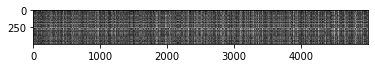
相关问题 1
观察距离矩阵的图形,可以发现某些行或者列的亮度更高。(注意:请使用默认的配色方案,颜色越黑表示距离越近,越白表示距离越远。)
- 数据中,导致出现明显亮行的原因是什么?
- 导致出现明显亮列的原因是什么?
答案:
- 明显亮行:说明这个测试用例与所有训练用例的差别都很大
- 明显亮列:说明存在训练用例与所有测试用例的差别都很大
# 现在,实现方法 predict_labels,并运行下列代码:
# 令 k = 1(最近邻)
y_test_pred = classifier.predict_labels(dists, k=1)

# 计算并打印正确率
num_correct = np.sum(y_test_pred == y_test)
accuracy = float(num_correct) / num_test
print('Got %d / %d correct => accuracy: %f' % (num_correct, num_test, accuracy))
Got 137 / 500 correct => accuracy: 0.274000
你应该能看到正确率大概为 27%。接下来尝试一下更大的 k 值,令 k = 5:
y_test_pred = classifier.predict_labels(dists, k=5)
num_correct = np.sum(y_test_pred == y_test)
accuracy = float(num_correct) / num_test
print('Got %d / %d correct => accuracy: %f' % (num_correct, num_test, accuracy))
Got 139 / 500 correct => accuracy: 0.278000
可以看到,结果会比 k = 1 的时候要好一点。
相关问题 2
我们也可以使用其它距离矩阵,如 L1 范式。 设在图片 $I_k$ 上坐标为 $(i,j)$ 的像素值为 $p _{ij}^{(k)}$,
所有图片的所有像素值的平均值(公共均值)为
$$ \mu=\frac{1}{nhw}\sum_{k=1}^n\sum_{i=1}^{h}\sum_{j=1}^{w}p_{ij}^{(k)} $$
所有图片中相同坐标的像素的平均值(像素均值)为
$$ \mu_{ij}=\frac{1}{n}\sum_{k=1}^np_{ij}^{(k)}. $$
公共标准差 $\sigma$ 和像素标准差 $\sigma_{ij}$ 的定义类似。
下面哪些预处理不会改变使用 L1 距离的最近邻分类器的运行结果:
- 减去公共均值 $\mu$ ($\tilde{p}{ij}^{(k)}=p{ij}^{(k)}-\mu$.)
- 减去像素均值 $\mu_{ij}$ ($\tilde{p}{ij}^{(k)}=p{ij}^{(k)}-\mu_{ij}$.)
- 减去公共均值 $\mu$ 然后除以公共标准差 $\sigma$.
- 减去像素均值 $\mu_{ij}$ 然后除以像素标准差 $\sigma_{ij}$.
- 旋转数据的坐标轴。
答:
上述处理都不会改变运行结果。
解释:
$$ L1(I_1, I_2) = \sum_p |I_1^p - I_2^p| $$
对于训练图像 X 和测试图像 y,相同坐标上的像素点 p 的像素值分比为 $I_x^p$ 和 $I_y^p$
变化 1,处理后的像素值为 $\tilde{I_x^p} = I_x^p -\mu$ 和 $\tilde{I_y^p} = I_y^p -\mu$,$\tilde{I_x^p} - \tilde{I_y^p} == I_x^p - I_y^p$,所以得到的距离矩阵都不会变。同理,变化 2 中相同坐标的像素点减去的值是相同的,距离矩阵也不会变,分类结果更不会变。
变化 3 ,处理后的像素值为 $\tilde{I_x^p} = \frac{I_x^p - \mu}{\sigma}$ 和 $\tilde{I_y^p} = \frac{I_y^p - \mu}{\sigma}$,最后的 L1 距离为 $L1 = \frac{1}{\sigma}\sum |I_x^p - I_y^p|$,由此可见,变化后只是所有图像的距离都变小了相同的倍数,距离矩阵与一个数 $\sigma$ 进行了除法运算,最后的分类结果不会改变(这是理论上的,但如果用整除的话还是会变的,非整除的话,由于浮点数运算误差的累加,还是可能出现不一样的结果)。
变化 4,处理后的像素值为 $\tilde{I_x^p} = \frac{I_x^p - \mu}{\sigma^p}$ 和 $\tilde{I_y^p} = \frac{I_y^p - \mu}{\sigma^p}$,最后 L1 距离为 $L1 = \sum \frac{|I_x^p - I_y^p|}{\sigma^p}$,这样看来这并不是一个线性变化,所以最后预测的结果可能会发生变化。
变化 5,处理之后,只是像素交换了坐标,同一位置上的像素集内部元素还是不变的,所以其实距离矩阵也不会变化,预测结果更不会变。
test_knn.ipynb 中对各种变换进行了实际的测试
# 接下来,我们使用部分向l量化,实现用单层循环来计算距离矩阵,
# 实现方法 compute_distances_one_loop,并运行如下代码:
dists_one = classifier.compute_distances_one_loop(X_test)

# 为了确认向量化结果的正确性,我们需要确保它的结果与简单方法一致。
# 判断两个矩阵相似的方法有很多,其中最简单的一种就是 F 范数。
# 两个矩阵的 F 范数是两个矩阵所有元素之差的平方和;
# 换句话说,就是把矩阵压成向量,然后计算他们的欧式距离。
difference = np.linalg.norm(dists - dists_one, ord='fro')
print('One loop difference was: %f' % (difference, ))
if difference < 0.001:
    print('Good! The distance matrices are the same')
else:
    print('Uh-oh! The distance matrices are different')
One loop difference was: 0.000000
Good! The distance matrices are the same
# 现在,在 compute_distance_no_loops 方法中实现全向量化版本的代码
# 并运行下列代码
dists_two = classifier.compute_distances_no_loops(X_test)

# 同样,通过计算两个矩阵的距离来验证结果
difference = np.linalg.norm(dists - dists_two, ord='fro')
print('No loop difference was: %f' % (difference, ))
if difference < 0.001:
    print('Good! The distance matrices are the same')
else:
    print('Uh-oh! The distance matrices are different')
(5000,)
No loop difference was: 0.000000
Good! The distance matrices are the same
# 比较一下不同实现的效率怎么样
def time_function(f, *args):
    """
    Call a function f with args and return the time (in seconds) that it took to execute.
    """
    import time
    tic = time.time()
    f(*args)
    toc = time.time()
    return toc - tic

two_loop_time = time_function(classifier.compute_distances_two_loops, X_test)
print('Two loop version took %f seconds' % two_loop_time)

one_loop_time = time_function(classifier.compute_distances_one_loop, X_test)
print('One loop version took %f seconds' % one_loop_time)

no_loop_time = time_function(classifier.compute_distances_no_loops, X_test)
print('No loop version took %f seconds' % no_loop_time)

# 你应该能看到使用全向量化方法之后性能明显提升了

# 注意:取决于你使用的机器
# 你可能会发现使用单层循序并没有性能的提升
# 相反还可能会更慢
Two loop version took 22.724715 seconds
One loop version took 39.343030 seconds
(5000,)
No loop version took 0.122352 seconds
交叉验证
我们已经实现了 kNN 分类器,但之前我们都是直接令 k = 5。现在我们来通过交叉验证来确定一下 k 的最佳取值。
num_folds = 5
k_choices = [1, 3, 5, 8, 10, 12, 15, 20, 50, 100]

X_train_folds = []
y_train_folds = []
################################################################################
# TODO:                                                                        #
# Split up the training data into folds. After splitting, X_train_folds and    #
# y_train_folds should each be lists of length num_folds, where                #
# y_train_folds[i] is the label vector for the points in X_train_folds[i].     #
# Hint: Look up the numpy array_split function.                                #
################################################################################
# *****START OF YOUR CODE (DO NOT DELETE/MODIFY THIS LINE)*****

X_train_folds = np.array_split(X_train, num_folds)
y_train_folds = np.array_split(y_train, num_folds)

# *****END OF YOUR CODE (DO NOT DELETE/MODIFY THIS LINE)*****

# A dictionary holding the accuracies for different values of k that we find
# when running cross-validation. After running cross-validation,
# k_to_accuracies[k] should be a list of length num_folds giving the different
# accuracy values that we found when using that value of k.
k_to_accuracies = {}


################################################################################
# TODO:                                                                        #
# Perform k-fold cross validation to find the best value of k. For each        #
# possible value of k, run the k-nearest-neighbor algorithm num_folds times,   #
# where in each case you use all but one of the folds as training data and the #
# last fold as a validation set. Store the accuracies for all fold and all     #
# values of k in the k_to_accuracies dictionary.                               #
################################################################################
# *****START OF YOUR CODE (DO NOT DELETE/MODIFY THIS LINE)*****
num_folds_count = np.ceil(X_train.shape[0]/num_folds)
for i in k_choices:
    list_acc = np.zeros(num_folds)
    for j in range(num_folds):
        start = int(j * num_folds_count)
        end = int((j+1) * num_folds_count)
        X_train_folds_train = np.delete(X_train,np.s_[start:end],0)
        y_train_folds_train = np.delete(y_train,np.s_[start:end],0)
        classifier.train(X_train_folds_train, y_train_folds_train)
        dists = classifier.compute_distances_no_loops(X_train_folds[j])
        y_test_pred = classifier.predict_labels(dists, k=i)
        num_correct = np.sum(y_test_pred == y_train_folds[j])
        accuracy = float(num_correct) / num_folds_count
        list_acc[j] = accuracy
    k_to_accuracies[i] = list_acc
# *****END OF YOUR CODE (DO NOT DELETE/MODIFY THIS LINE)*****

# Print out the computed accuracies
for k in sorted(k_to_accuracies):
    for accuracy in k_to_accuracies[k]:
        print('k = %d, accuracy = %f' % (k, accuracy))
k = 1, accuracy = 0.263000
k = 1, accuracy = 0.257000
k = 1, accuracy = 0.264000
k = 1, accuracy = 0.278000
k = 1, accuracy = 0.266000
k = 3, accuracy = 0.239000
k = 3, accuracy = 0.249000
k = 3, accuracy = 0.240000
k = 3, accuracy = 0.266000
k = 3, accuracy = 0.254000
k = 5, accuracy = 0.248000
k = 5, accuracy = 0.266000
k = 5, accuracy = 0.280000
k = 5, accuracy = 0.292000
k = 5, accuracy = 0.280000
k = 8, accuracy = 0.262000
k = 8, accuracy = 0.282000
k = 8, accuracy = 0.273000
k = 8, accuracy = 0.290000
k = 8, accuracy = 0.273000
k = 10, accuracy = 0.265000
k = 10, accuracy = 0.296000
k = 10, accuracy = 0.276000
k = 10, accuracy = 0.284000
k = 10, accuracy = 0.280000
k = 12, accuracy = 0.260000
k = 12, accuracy = 0.295000
k = 12, accuracy = 0.279000
k = 12, accuracy = 0.283000
k = 12, accuracy = 0.280000
k = 15, accuracy = 0.252000
k = 15, accuracy = 0.289000
k = 15, accuracy = 0.278000
k = 15, accuracy = 0.282000
k = 15, accuracy = 0.274000
k = 20, accuracy = 0.270000
k = 20, accuracy = 0.279000
k = 20, accuracy = 0.279000
k = 20, accuracy = 0.282000
k = 20, accuracy = 0.285000
k = 50, accuracy = 0.271000
k = 50, accuracy = 0.288000
k = 50, accuracy = 0.278000
k = 50, accuracy = 0.269000
k = 50, accuracy = 0.266000
k = 100, accuracy = 0.256000
k = 100, accuracy = 0.270000
k = 100, accuracy = 0.263000
k = 100, accuracy = 0.256000
k = 100, accuracy = 0.263000
# plot the raw observations
for k in k_choices:
    accuracies = k_to_accuracies[k]
    plt.scatter([k] * len(accuracies), accuracies)

# plot the trend line with error bars that correspond to standard deviation
accuracies_mean = np.array([np.mean(v) for k,v in sorted(k_to_accuracies.items())])
accuracies_std = np.array([np.std(v) for k,v in sorted(k_to_accuracies.items())])
plt.errorbar(k_choices, accuracies_mean, yerr=accuracies_std)
plt.title('Cross-validation on k')
plt.xlabel('k')
plt.ylabel('Cross-validation accuracy')
plt.show()
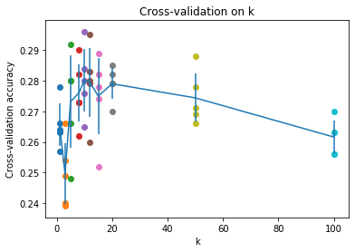
# Based on the cross-validation results above, choose the best value for k,
# retrain the classifier using all the training data, and test it on the test
# data. You should be able to get above 28% accuracy on the test data.
best_k = 10

classifier = KNearestNeighbor()
classifier.train(X_train, y_train)
y_test_pred = classifier.predict(X_test, k=best_k)

# Compute and display the accuracy
num_correct = np.sum(y_test_pred == y_test)
accuracy = float(num_correct) / num_test
print('Got %d / %d correct => accuracy: %f' % (num_correct, num_test, accuracy))
Got 141 / 500 correct => accuracy: 0.282000
相关问题 3
相同的分类器配置下,对于所有的 $k$,下面关于 $k$-近邻($k$-NN)的说法正确的有哪些?
- k-NN 分类器的决策边界是线性的;
- 1-NN 的训练误差总是比 5-NN 的要低;
- 1-NN 的测试误差总是要比 5-NN 要低;
- 用 k-NN 分类器对一个测试用例进行分类,所需要的时间随着训练集大小的增大而变长;
- 以上全都不对。
答案:
2 和 4
理由:
- 1:k-NN 的决策边界一般不会是线性的,它是一种非线性的分类器
- 2:1-NN 总是找与目标图像差距最小的图片,在训练集上进行分类的话,肯定会找到原图,所以训练误差是 0%;而 5-NN 的话,显然不会是 0;
- 3:这个不一定,可能出现意外;
- 4:k-NN 要计算测试用例与训练集所有图片的距离,所以训练集越大就越慢;